Fast Gantt Chart with Excel

Make a useful Gantt chart with Excel in only 3 simple steps

Reading Time: 5 minutes

Post published on 26/05/2021 by Fabrizio Cesarini on site https://www.fabriziocesarini.com and released with licenza CC BY-NC-ND 3.0 IT (Creative Common – Attribuzione – Non commerciale – Non opere derivate 3.0 Italia)

Cover Image credits and copyrights by XPS on Unsplash https://unsplash.com/@xps

Article Images credits and copyrights by Fabrizio Cesarini https://www.fabriziocesarini.com

Excel can be used in an infinite number of ways to do the most diverse things and sometimes it lends itself well to uses a little … less standard.

We can also use Excel making use of small tricks that can make us get simple and quick solutions but, at the same time, functional. Sometimes it is not necessary to create a complex work tool, but instead it is necessary to create a simple and functional tool that is well suited to the purpose. In these cases the speed factor is absolutely fundamental.

Let’s take the case of having to manage a simple project. As you know I’ve been involved in project management for many years and I’ve already explained in a previous article how to create a Gantt chart suitable for the purpose. I love the Gantt chart especially for its visual immediacy.

The problem is that to create a Gantt chart I have to use a project management software that most of the time is very complex to use. There are some excellent ones, both paid and free, but they all share the same problem. They are complex to use because it is very difficult to minimize the inherent complexity of project representation.

This is precisely why I explained in an article how to create a Gantt chart with Excel. If you missed it you can go read it here.

However, if you are in the very frequent situation of having to manage a project composed of a few simple tasks and you don’t want to bother with complex procedures but also don’t want to create an ad hoc spreadsheet you can use a trick that I personally love.

With just 3 simple steps we can quickly create a simple and functional Gantt chart with Excel.

Let’s get started!

Step 1 – Data Table Creation

Let’s open the Excel sheet and add 5 columns

Task
Start
Finish
Duration
Bar

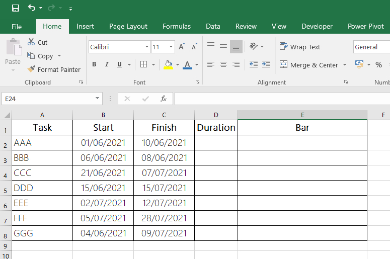
The Task column will contain the list of tasks indicated by their name. The Start column will show the start dates of the various tasks and the Finish column will show their end dates. The Duration column will show the number of days of the tasks. Finally, the Bar column will contain the bars of our Gantt chart.

Now go and add as many and as many tasks as you want (you need) indicating for each of them the start and end date.

In figure 1 you can see an example of a table with data created ad hoc for this article.

Article Fast Gantt Chart with Excel - Fig 1 - Data Table — Fig 1 – Data Table

Step 2 – Calculations

Now let’s move on to the calculations. Actually this is only one calculation.

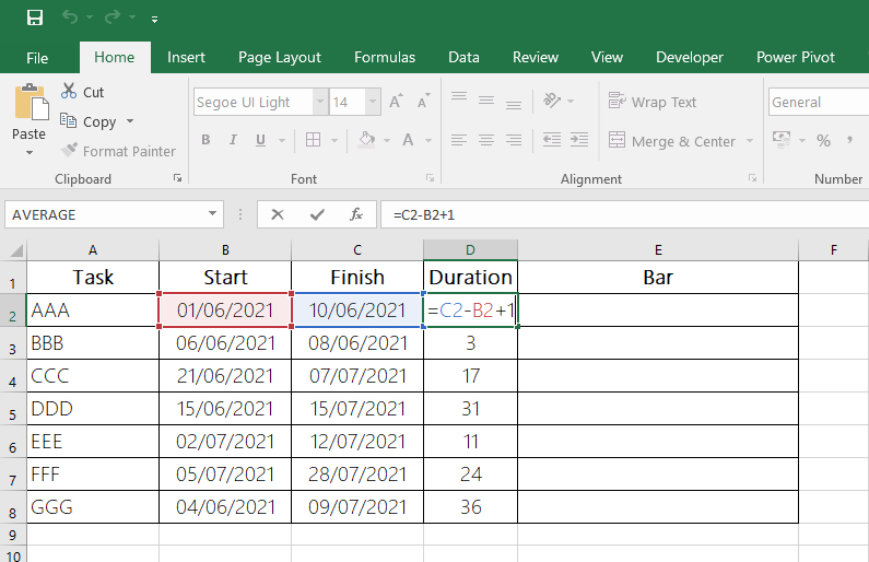
We need to fill the Duration column with the number of days that represent the duration of the task starting from the start date until the end date.

To do this we simply need to enter a simple formula:

Duration = Start Date – End Date + 1

The plus one server to take into account the day on which the task starts otherwise the duration would be shorter than one day.

Referring to the data shown in the table in Figure 1, it will be enough to insert in cell D2 the following formula

=C2-B2+1

Once the formula has been created, copy and paste (or simply drag and drop) the formula into the other cells to calculate all the other durations.

You can see the result in figure 2

Article Fast Gantt Chart with Excel - Fig 2 - Duration Calculation — Fig 2 – Duration Calculation

Step 3 – Creating the Bars

We have arrived at the third and final step.

In the Bar column we need to create horizontal bars whose length is equal to the duration of the tasks.

You would think that we need to insert a chart inside the cell. But no, that would be too complicated.

It is here that we need to use a simple trick.

In order to do this, let’s use a little known Excel function…REPT.

The REPT function repeats a character a certain number of times.

Its syntax is as follows:

REPT(text_to_repeat; number_times_to_repeat_text)

The REPT function syntax has the following arguments:

text_to_repeat The text you want to repeat
number_times_to_repeat_text A positive number specifying the number of times to repeat text.

We’ll use this function to make a particular character write a number of times equal to duration.

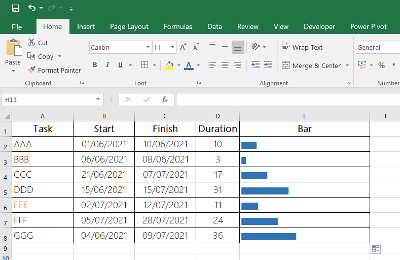
Therefore, always referring to the data shown in Figure 1, in cell E2 we will insert the following function

=REPT(“|”;D2)

This function will write the character | as many times as the number present in cell D2 (Duration). We copy and paste the function in the other cells as well.
Before proceeding further we need to make a simple but fundamental change to the cells that contain the bars. We need to set a particular font. We need to use a font that can best represent the vertical bar font to suit our purpose. To do this we select the font “Britannic Bold“. You can also select any size you like and a color you prefer instead of the normal black. In my case I chose a particular shade of blue.

What we will get is a table with a series of bars indicating the duration of the task as you can see in figure 3.

Article Fast Gantt Chart with Excel - Fig 3 - Duration Bars — Fig 3 – Duration Bars

I know what you’re thinking. But this is not a Gantt! That’s right. The bars indicate durations but they are not positioned correctly. In fact, the bars should be positioned with the start date in mind so that they are perfectly readable.

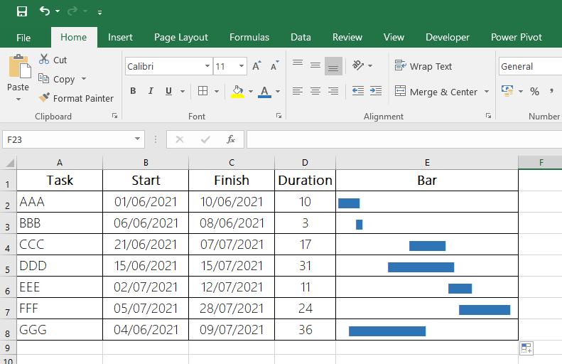
Nothing complicated. To do this we simply need to make a small change to the formula to make it take into account the start date.

What we need to do is to insert in the cell as many empty bars in front of the duration bar in a number equal to the number of days from the start date to the first date in the project.

The formula present in cell E2 will become the following:

=REPT(” “;B2-MIN(B$2:B$8)) & REPT(“|”;D2)

We have simply added REPT(” “;B2-MIN(B$2:B$8)) to the previous formula and the result is hooked into the other text using the & character.

This function adds as many empty bars, in front of the colored bar, as many days have passed from the start date of the task (e.g. B2) to the lesser date (B2:B8).